
BigQuery for Beginners: Query Billions of Rows for Free
What you build: SQL on a public dataset with millions of rows, then your own sales table with a view and a daily partition, in your own Google Cloud account. Every step tested.

✍️ Translate this blog into Hindi, Tamil or Telugu
In this lab you run SQL on a public table with millions of rows, then build your own small sales dataset in BigQuery: you load a CSV file, query it, save a view, split a table by day and see how that cuts the bytes a query reads. You finish by deleting everything.
Who it is for: beginners who know a little SQL (SELECT, GROUP BY) or none at all. Time: about 1 hour. Cost: free tier (BigQuery gives every account 1 TB of query reading and 10 GB of storage each month at no charge; this whole lab reads well under 1 GB).
Every command below was run for real by the CareerByteCode Team on a fresh Google Cloud project, and every output and screenshot is the real result we got. We ran the commands from a terminal with the Google Cloud CLI (gcloud and bq); Cloud Shell in your browser has the same tools ready, so you can copy and paste each command there.
⭐ Recommended by CareerByteCode · BytePlay courseNVIDIA GPU AI Factory: Architecture, Engineering & Operations₹40,000Start learning →Part A: BigQuery in plain English
BigQuery is Google's data warehouse: a place to keep large tables and ask questions about them with SQL. You do not create servers, disks or clusters. You load data, you write a query, and Google runs it on many machines at once.

Five words you will use in this lab:
- Project: your Google Cloud account space. Every dataset lives inside one project. Real-life example: a house that holds everything you own on Google Cloud.
- Dataset: a folder for tables and views. Real-life example: one cupboard in that house, with a name on the door (we call ours
cbc_lab). - Table: rows and columns, like a spreadsheet tab. BigQuery stores each column on its own, so a query that names 2 columns reads only those 2.
- View: a saved query that behaves like a table. Real-life example: a bookmark that always opens the latest version of a report.
- Partitioned table: a table split into parts (here one part per day). A query that asks for one day reads only that part. Real-life example: a filing cabinet with one drawer per day; you open one drawer, not the whole cabinet.
How you pay: with on-demand pricing you pay for the bytes a query reads, and the first 1 TB each month is free. That is why we use --dry_run before big queries: it tells you the bytes without running anything.
Before you start
- A Google Cloud account (the free trial works) and a project with billing linked. Create one at https://console.cloud.google.com/projectcreate if you do not have one.
- Open Cloud Shell (the
>_icon at the top right of the Google Cloud console). It already hasgcloudandbq. - Save your project id in a variable. Replace the text in quotes with your own project id:
export PROJECT_ID="your-project-id"- The BigQuery API is on by default in new projects. If a command says it is disabled, run
gcloud services enable bigquery.googleapis.com.
Part B: the lab
Step 1: point the CLI at your project
Why: every bq command runs against the "current" project. Setting it once saves typing it in every command.
gcloud config set project $PROJECT_ID
bq version
Expected output (the version may be newer for you):
Updated property [core/project].
This is BigQuery CLI 2.1.42
Step 2: your first query on a public dataset
Why: Google keeps free public datasets you can query from any project. usa_names lists baby names in the USA from 1910 to 2013. This query adds up how many babies got each name and shows the top 5.
bq query --use_legacy_sql=false \
"SELECT name, SUM(number) AS total
 FROM \`bigquery-public-data.usa_names.usa_1910_2013\`
 GROUP BY name ORDER BY total DESC LIMIT 5"
Real output:
+---------+---------+
|  name   |  total  |
+---------+---------+
| James   | 4942431 |
| John    | 4834422 |
| Robert  | 4718787 |
| Michael | 4297230 |
| William | 3822209 |
+---------+---------+
What each part means:
bq queryruns a query.--use_legacy_sql=falseasks for standard SQL (the normal SQL you know).- The table name in backticks is
project.dataset.table: here the project isbigquery-public-data. GROUP BY namemakes one row per name;SUM(number)adds the counts;ORDER BY total DESC LIMIT 5keeps the 5 biggest.
Step 3: dry run, see the bytes before you pay
Why: a dry run checks your SQL and tells you how many bytes it would read, without running it and without any charge.
bq query --use_legacy_sql=false --dry_run \
"SELECT name, SUM(number) AS total
 FROM \`bigquery-public-data.usa_names.usa_1910_2013\`
 GROUP BY name ORDER BY total DESC LIMIT 5"
Query successfully validated. Assuming the tables are not modified, running this query will process 88145726 bytes of data.Now ask for one column only:
bq query --use_legacy_sql=false --dry_run \
"SELECT name FROM \`bigquery-public-data.usa_names.usa_1910_2013\` LIMIT 5"
Query successfully validated. Assuming the tables are not modified, running this query will process 43726110 bytes of data.
The first query reads two columns (name and number), about 88 MB. The second reads one column, about 43 MB: half. LIMIT 5 does not make it cheaper, because BigQuery still reads the whole column before it cuts the result. Lesson: never write SELECT * on a big table; name only the columns you need.
Step 4: create your own dataset
Why: your tables need a home. --location=US decides where the data is stored; keep all datasets you join together in the same location.
bq --location=US mk --dataset --description "CareerByteCode BigQuery lab" $PROJECT_ID:cbc_lab
bq ls
Dataset 'your-project-id:cbc_lab' successfully created.
datasetId
-----------
cbc_labStep 5: make a small sales file
Why: a tiny CSV file so you can see every number with your own eyes. Each row is one order in one city.
cat > sales.csv <<EOF
order_id,order_date,city,product,qty,price
1,2026-11-01,Chennai,Notebook,3,120.00
2,2026-11-01,Bengaluru,Pen,10,15.50
3,2026-11-02,Chennai,Backpack,1,1450.00
4,2026-11-02,Hyderabad,Notebook,5,120.00
5,2026-11-03,Bengaluru,Backpack,2,1450.00
6,2026-11-03,Chennai,Pen,20,15.50
7,2026-11-04,Hyderabad,Pen,8,15.50
8,2026-11-04,Bengaluru,Notebook,4,120.00
EOF
cat sales.csv
Step 6: load the file into a table
Why: bq load copies the file into a BigQuery table. The last line is the schema: the name and type of each column (INTEGER, DATE, STRING, NUMERIC). --skip_leading_rows=1 skips the header row.
bq load --source_format=CSV --skip_leading_rows=1 \
  cbc_lab.sales ./sales.csv \
  order_id:INTEGER,order_date:DATE,city:STRING,product:STRING,qty:INTEGER,price:NUMERIC
bq show --schema --format=prettyjson cbc_lab.sales
The schema BigQuery saved (end of the output):
Upload complete.

Waiting on bqjob_r795a0428526285ad_000001a1eb7a1560_1 ... (0s) Current status: RUNNING

Waiting on bqjob_r795a0428526285ad_000001a1eb7a1560_1 ... (0s) Current status: DONE
[
  {
    "mode": "NULLABLE",
    "name": "order_id",
    "type": "INTEGER"
  },
  {
    "mode": "NULLABLE",
    "name": "order_date",
    "type": "DATE"
  },
  {
    "mode": "NULLABLE",
    "name": "city",
    "type": "STRING"
  },
  {
    "mode": "NULLABLE",
    "name": "product",
    "type": "STRING"
  },
  {
    "mode": "NULLABLE",
    "name": "qty",
    "type": "INTEGER"
  },
  {
    "mode": "NULLABLE",
    "name": "price",
    "type": "NUMERIC"
  }
]
Step 7: peek at the rows
Why: bq head shows a few rows without running a query, so it reads nothing billable.
bq head -n 5 cbc_lab.sales+----------+------------+-----------+----------+-----+-------+
| order_id | order_date | city | product | qty | price |
+----------+------------+-----------+----------+-----+-------+
| 3 | 2026-11-02 | Chennai | Backpack | 1 | 1450 |
| 5 | 2026-11-03 | Bengaluru | Backpack | 2 | 1450 |
| 2 | 2026-11-01 | Bengaluru | Pen | 10 | 15.5 |
| 6 | 2026-11-03 | Chennai | Pen | 20 | 15.5 |
| 7 | 2026-11-04 | Hyderabad | Pen | 8 | 15.5 |
+----------+------------+-----------+----------+-----+-------+
In the console you can see the same table under your project: open BigQuery > Studio, then expand your project > cbc_lab > sales. The Schema tab shows the 6 columns and the Preview tab shows the rows:


Step 8: revenue by city
Why: this is the kind of question a manager asks every day: which city sells the most? qty * price gives the value of each order and SUM adds them per city.
bq query --use_legacy_sql=false \
"SELECT city, SUM(qty * price) AS revenue, COUNT(*) AS orders
 FROM cbc_lab.sales GROUP BY city ORDER BY revenue DESC"
+-----------+---------+--------+
| city | revenue | orders |
+-----------+---------+--------+
| Bengaluru | 3535 | 3 |
| Chennai | 2120 | 3 |
| Hyderabad | 724 | 2 |
+-----------+---------+--------+Check it by hand: Bengaluru has 10 pens at 15.50 (155), 2 backpacks at 1450 (2900) and 4 notebooks at 120 (480). 155 + 2900 + 480 = 3535. The query is right.
Step 9: save the query as a view
Why: a view stores the SQL, not the data. Anyone can now run SELECT * FROM cbc_lab.city_revenue and always get the latest numbers from the sales table.
bq mk --use_legacy_sql=false \
  --view "SELECT city, SUM(qty * price) AS revenue FROM \`$PROJECT_ID.cbc_lab.sales\` GROUP BY city" \
  cbc_lab.city_revenue
bq query --use_legacy_sql=false "SELECT * FROM cbc_lab.city_revenue ORDER BY revenue DESC"
View 'your-project-id:cbc_lab.city_revenue' successfully created.
+-----------+---------+
| city | revenue |
+-----------+---------+
| Bengaluru | 3535 |
| Chennai | 2120 |
| Hyderabad | 724 |
+-----------+---------+
Step 10: a partitioned table (one part per day)
Why: real sales tables grow every day. If the table is split by order_date, a query for one day reads only that day's part.
bq query --use_legacy_sql=false \
"CREATE TABLE cbc_lab.sales_by_day
 PARTITION BY order_date AS
 SELECT * FROM cbc_lab.sales"
bq show --format=prettyjson cbc_lab.sales_by_day | grep -A3 timePartitioning
Waiting on bqjob_rff8b96dd26827be_000001a1eb7ae2d5_1 ... (0s) Current status: RUNNING
Waiting on bqjob_rff8b96dd26827be_000001a1eb7ae2d5_1 ... (0s) Current status: DONE
Created your-project-id.cbc_lab.sales_by_day
"timePartitioning": {
"field": "order_date",
"type": "DAY"
},The timePartitioning block confirms: one part per DAY, on the order_date column.
POC: prove the partition filter reads less
Run two dry runs on the partitioned table: the whole table, then one day.
bq query --use_legacy_sql=false --dry_run "SELECT * FROM cbc_lab.sales_by_day"
bq query --use_legacy_sql=false --dry_run "SELECT * FROM cbc_lab.sales_by_day WHERE order_date = \"2026-11-03\""
Query successfully validated. Assuming the tables are not modified, running this query will process 467 bytes of data.
Query successfully validated. Assuming the tables are not modified, running this query will process 115 bytes of data.
Proof: the whole table is 467 bytes and one day is 115 bytes, about a quarter, because our data has 4 days. On a table with 3 years of data, the same filter would read 1 day out of about 1,100. That is the single biggest saving in BigQuery.
Break it and fix it
Beginners often type a column name that does not exist. Let us do it on purpose: we ask for town, but the column is called city.
bq query --use_legacy_sql=false "SELECT town, SUM(qty) FROM cbc_lab.sales GROUP BY town"Error in query string: Error processing job 'your-project-id:bqjob_r29bf9e42e8c34cc2_000001a1eb7b6cdc_1': Unrecognized name: town
at [1:8]The error says exactly what is wrong: Unrecognized name: town at line 1, character 8. Fix: look at the schema, then use the real name.
bq show --schema cbc_lab.sales
bq query --use_legacy_sql=false "SELECT city, SUM(qty) AS items FROM cbc_lab.sales GROUP BY city ORDER BY items DESC"
[{"name":"order_id","type":"INTEGER","mode":"NULLABLE"},{"name":"order_date","type":"DATE","mode":"NULLABLE"},{"name":"city","type":"STRING","mode":"NULLABLE"},{"name":"product","type":"STRING","mode":"NULLABLE"},{"name":"qty","type":"INTEGER","mode":"NULLABLE"},{"name":"price","type":"NUMERIC","mode":"NULLABLE"}]
+-----------+-------+
| city | items |
+-----------+-------+
| Chennai | 24 |
| Bengaluru | 16 |
| Hyderabad | 13 |
+-----------+-------+
Clean up (delete everything)
Why: stored tables cost a little each month after the free 10 GB, and an empty project is easier to read. bq rm -r -f -d removes the dataset with every table and view inside it, without asking.
bq rm -r -f -d cbc_lab
bq ls
echo "datasets left: $(bq ls --format=json | grep -c datasetId)"
datasets left: 0
datasets left: 0 is your proof. Public datasets were never copied into your project, so there is nothing else to delete.
FAQ
Is BigQuery really free for this lab? Yes. Each month the first 1 TB of query reading and the first 10 GB of storage are free. This lab reads about 0.2 GB in total and stores a few kilobytes for a few minutes.
What is the BigQuery sandbox? A way to use BigQuery without a billing account. It has the same free limits, but tables expire after 60 days. Everything in this lab works in the sandbox too.
Why does LIMIT not reduce the bytes? BigQuery reads the columns first and cuts the rows at the end. Use fewer columns, a partition filter, or a smaller table to read less.
Do I need to learn a new kind of SQL? No. Standard SQL in BigQuery is the SQL you know, with extras like backticks around project.dataset.table names.
What is the difference between a table and a view? A table stores data. A view stores only the query and runs it each time you use it.
Can I load data from Google Sheets or Cloud Storage? Yes. bq load also accepts files in Cloud Storage (gs://...), and the console can link a Google Sheet as a table.
Where does BigQuery store my data? In the location you choose when you create the dataset (here US). You cannot move a dataset later; you copy it instead.
Troubleshooting
| You see | Why | Fix |
|---|---|---|
BigQuery API has not been used in project | The API is off | gcloud services enable bigquery.googleapis.com |
Not found: Dataset ...:cbc_lab | Wrong project, or the dataset was deleted | gcloud config set project $PROJECT_ID, then run Step 4 again |
Unrecognized name: ... | A column name is wrong | bq show --schema cbc_lab.sales and use the exact name |
Could not parse '...' as DATE | A date in the CSV is not YYYY-MM-DD | Fix the file, then load it again with --replace |
Access Denied: ... bigquery.jobs.create | Your account cannot run jobs in this project | Ask the project owner for the BigQuery User role |
| Query reads far more bytes than expected | SELECT * or no partition filter | Name the columns, filter on the partition column |
What next
- Read our tested Kubernetes lab: Zero to Kubernetes in 2.5 hours.
- More hands-on posts from the community: ByteBlog.
- Practice with guided projects in ByteLabs and see the full courses.
Prepared by the CareerByteCode Team from our tested lab, with AI help for the write-up.
⭐ Keep learning with CareerByteCode
Hand-picked to go deeper on this topicGet CareerByteCode Team's next blog by email
One email a week when they publish. Add the weekly Best of ByteBlog too. No spam, unsubscribe with one click.
We email you once to confirm. By subscribing you agree to the privacy policy.
Related blogs
 CareerByteCode Team
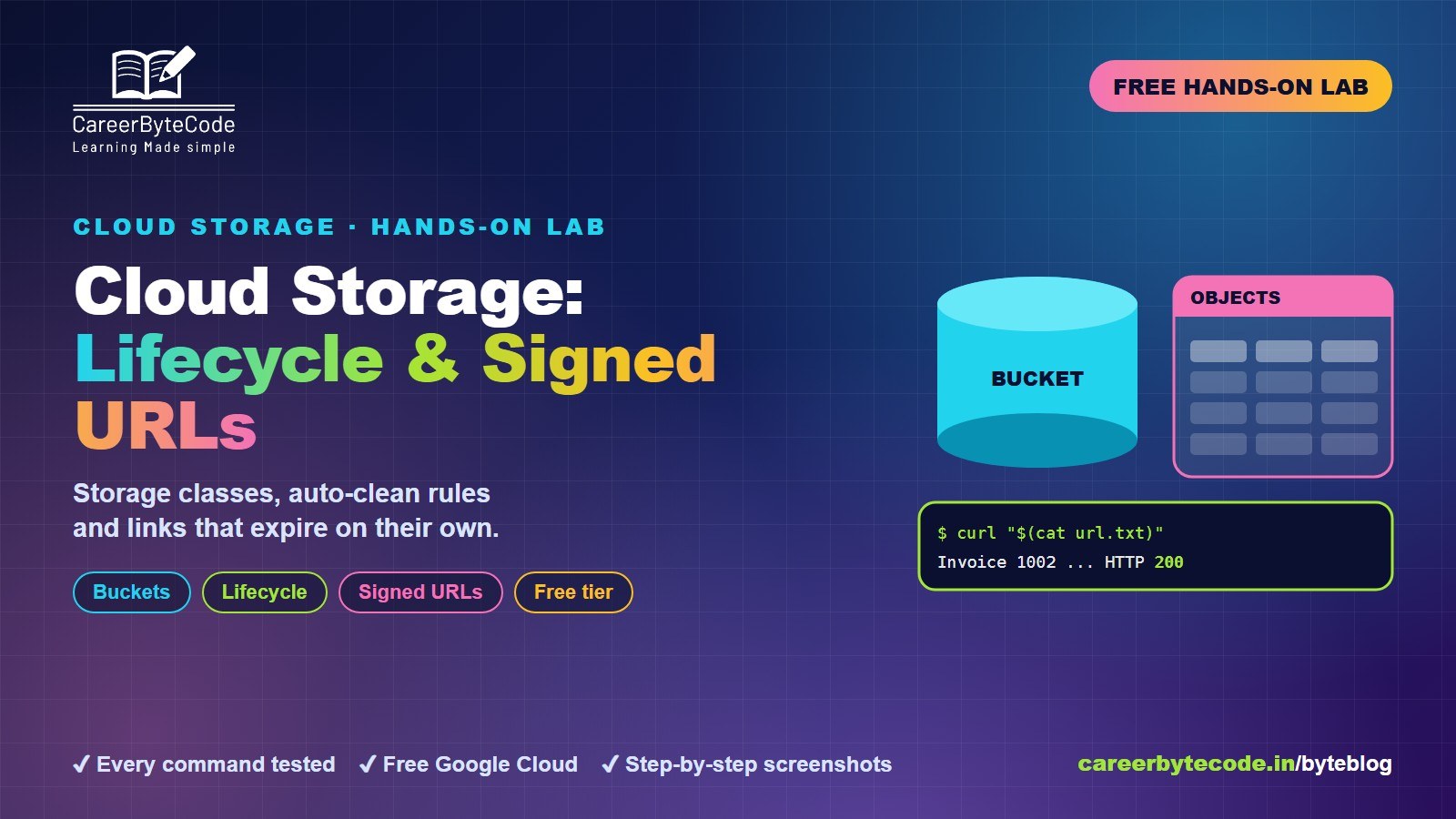
Cloud Storage Deep Dive: Classes, Lifecycle and Signed URLs
What you build: a private bucket with storage classes, a lifecycle policy, object versions and expiring signed URLs, in your own Google Cloud account. Every step tested.
#beginners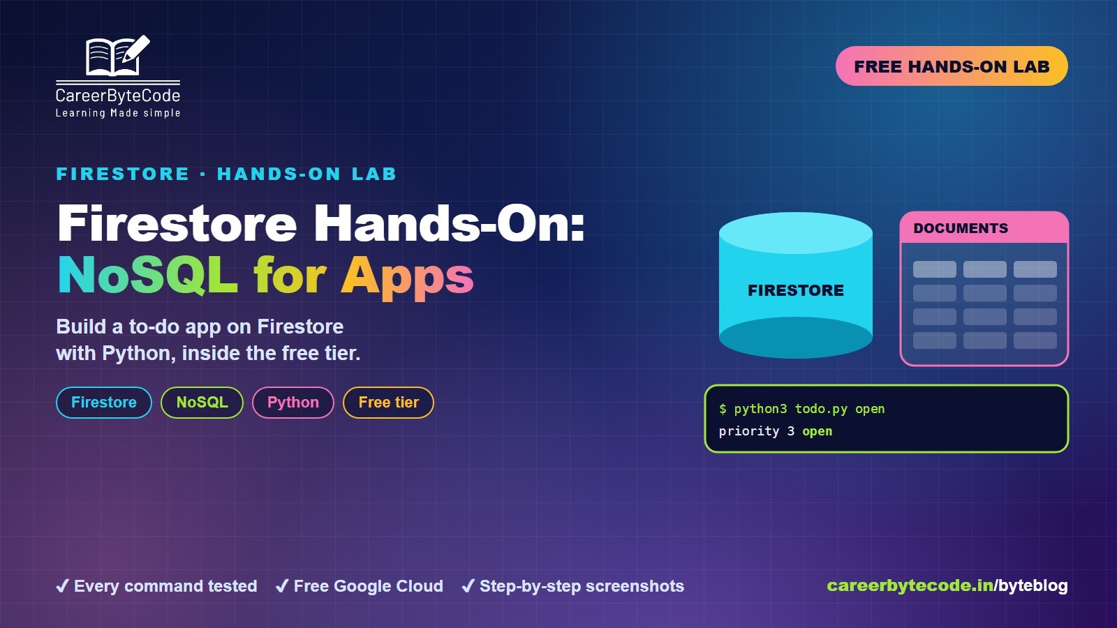 CareerByteCode Team
Firestore Hands-On: A NoSQL Database for Apps
What you build: a to-do app on Firestore in the free tier, in your own Google Cloud account. Every step, command and screenshot explained for beginners.
#bigquery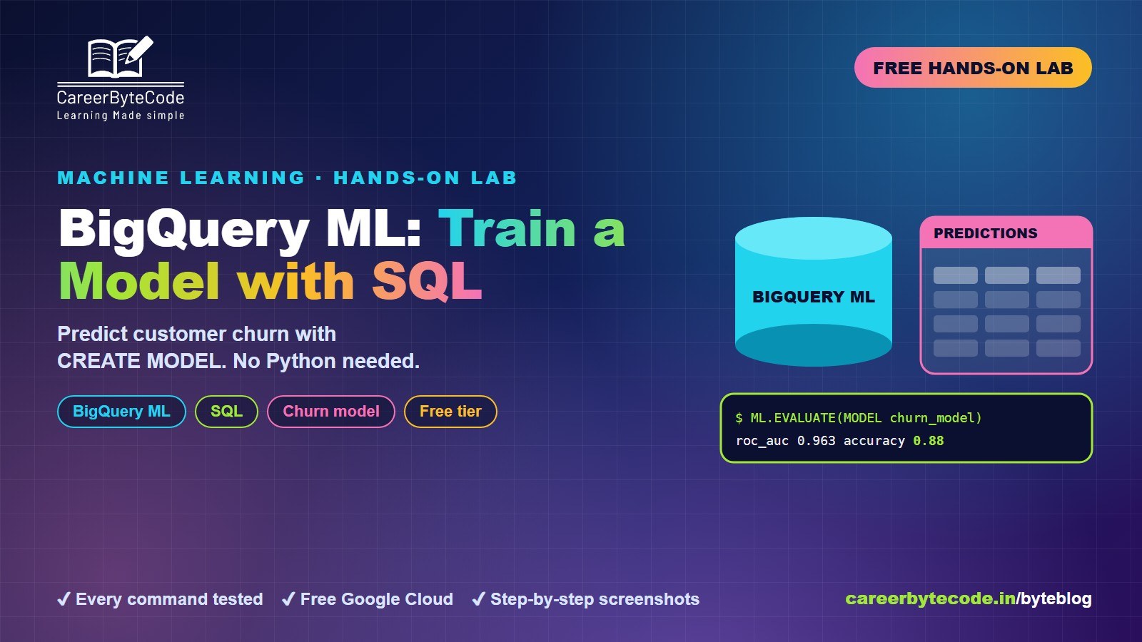 CareerByteCode Team
BigQuery ML: Train a Model with Just SQL
What you build: a churn prediction model written in SQL with BigQuery ML, scored and used for predictions, in your own Google Cloud account. Every step tested.
#beginners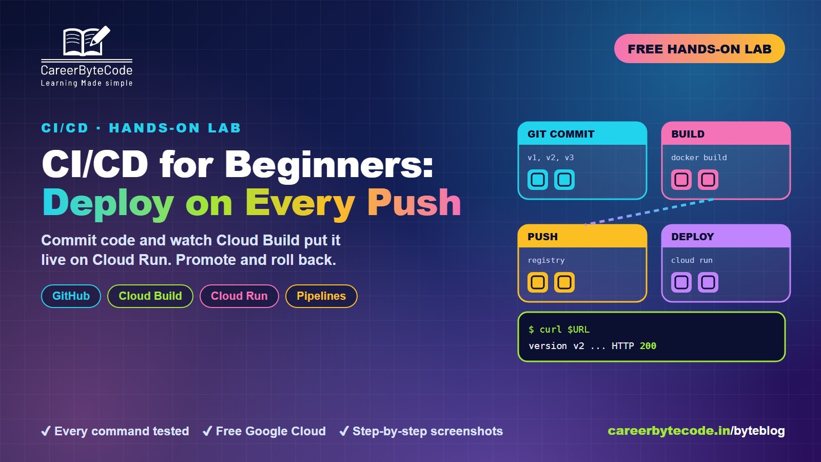 CareerByteCode Team
CI/CD for Beginners: Build and Deploy on Every Git Push
What you build: a pipeline from a git commit to a live Cloud Run app, with a test address, one-command promote and rollback, in your own Google Cloud account. Every step tested.
💬 Comments (0)
Top · NewestSign in to comment